
Credit Scoring Series Part Five: Credit Scorecard Development
Credit scorecard development describes how to turn data into a scorecard model, assuming that data preparation and the initial variable selection process (filtering) have been completed, and a filtered training dataset is available for the model building process. The development process consists of four main parts: variable transformations, model training using logistic regression, model validation, and scaling.

Figure 1. Standard scorecard development process
Variable Transformations for Credit Scorecards
A standard credit scorecard model, based on logistic regression, is an additive model; hence, special variable transformations are required. The commonly adopted transformations – fine classing, coarse classing, and either dummy coding or weight of evidence (WOE) transformation – form a sequential process that provide a model outcome that’s both easy to implement and explain. Additionally, these transformations help convert non-linear relationships between independent variables and the dependent variable into a linear relationship – which is the customer behavior most organizations are after. We’ll briefly explain the four types of common transformations below.
Fine classing - Applied to all continuous variables and discrete variables with high cardinality. This is the process of initial binning into typically between 20 and 50 fine granular bins.
Coarse classing - Where a binning process is applied to the fine granular bins to merge those with similar risk and create fewer bins, usually up to ten. The purpose of coarse classing is to create fewer, simpler bins with distinctive risk factors while minimizing information loss. However, to create a robust model that’s resistant to overfitting, each bin should contain a sufficient number of observations from the total account (usually a minimum amount of 5%). These opposing goals can be achieved through an optimization in the form of optimal binning that maximizes a variable’s predictive power during the coarse classing process. Optimal binning utilizes the same statistical measures used during variable selection, such as information value, Gini and chi-square statistics. The most popular measure is, again, information value, although a combination of two or more measures is often beneficial. The missing values, if they contain predictive information, should be a separate class or merged in a bin with similar risk factors.
Dummy coding - This is the process of creating binary (dummy) variables for all coarse classes except the reference class. This approach may present issues since extra variables require more memory and processing resources, and because overfitting may occur due to the reduced degrees of freedom.
Weight of evidence (WOE) transformation - This is the alternative (and often preferred) approach to dummy coding that substitutes each coarse class with a risk value and collapses the risk values into a single numeric variable. The numeric variable describes the relationship between an independent variable and a dependent variable. The WOE framework is well suited for logistic regression modeling since both are based on log-odds calculation. In addition, WOE transformation standardizes all independent variables; as such, users can directly compare the parameters in a subsequent logistic regression. The main drawback of this approach is that it only considers the relative risk of each bin without considering the proportion of accounts in each bin. The information value can be utilized instead to assess the relative contribution of each bin.
Keep in mind both dummy coding and WOE transformation yield similar results – which option to use mainly depends on a data scientist’s preference.
But be warned – optimal binning, dummy coding and WOE transformation are time-consuming processes when carried out manually. That’s why a software package for binning, optimization, and WOE transformation is extremely useful.
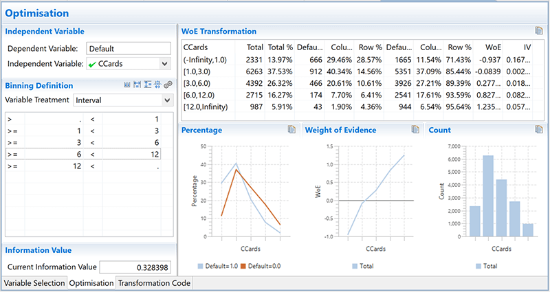
Figure 2. Automated optimal binning and WOE transformation with WPS software
Model Training and Scaling
Logistic regression is commonly used in credit scoring for solving binary classification problems. Prior to model fitting, another iteration of variable selection is valuable to check if the newly WOE-transformed variables are still good model candidates. Preferred candidate variables are those with higher information value (usually between 0.1 and 0.5), have a linear relationship with the dependent variable, have good coverage across all categories, have a normal distribution, contain a notable overall contribution, and are relevant to the business.
Many analytics vendors include the logistic regression model in their software products with an extensive range of statistical and graphical functions. For example, the implementation of the SAS language PROC LOGISTIC in WPS offers a comprehensive set of options for automated variable selection, restriction of model parameters, weighted variables, obtaining separate analysis for different segments, scoring on a different dataset, generating automated deployment code, and more.
Once the model has been aligned, the next step is to adjust the model to a scale the business desires. This is called scaling. Scaling is a measuring instrument that makes scores across different credit scorecards consistent and standardized. The minimum and maximum score values and the score range help in risk interpretation and should be reported to the business; often, businesses require teams to use the same score range for multiple credit scorecards so they all have the same risk interpretation.
A popular scoring method logarithmically creates discrete scores, where the odds double at a pre-determined number of points. This requires specifying the three parameters: base points such as 600 points, base odds (50:1, for example), and points to double the odds, (20, for example). Score points correspond to each of the bins of model variables, while the model intercept is translated into the base points. The scaling output with tabulated allocation of points represents the actual credit scorecard model.

Figure 3. Scorecard scaling
Model Performance
Model assessment is the final step in the model building process. It consists of three distinctive phases: evaluation, validation, and acceptance.
Evaluation for accuracy: The first question to ask in order to test the model is, Did I build the model right? The key metrics to assess are statistical measures including model accuracy, complexity, error rate, model fitting statistics, variable statistics, significance values, and odds ratios.
Evaluation for robustness: The next question to ask is, Did I build the right model? when moving from classification accuracy and statistical assessment towards ranking ability and business assessment.
The choice of validation metrics depends on type of the model classifier. The most common metrics for binary classification problems are gains chart, lift chart, ROC curve and Kolmogorov-Smirnov chart. The ROC curve is the most common multi-purpose tool for visualizing model performance, and is also used in:
- Champion-challenger methodology to choose the best performing model;
- Testing model performance on unseen data and comparing it to the training data; and
- Selecting optimal thresholds, which maximizes the true positive rate, while minimizing the false positive rate
The ROC curve is created by plotting sensitivity against probability of false alarm (false positive rate) at different thresholds. Assessing performance metrics at different thresholds is a desirable feature of the ROC curve. Different types of business problems will have different thresholds based on their business strategy.
The area under the ROC curve (AUC) is a useful measure that indicates a classifier’s predictive ability. In credit risk, an AUC of 0.75 or higher is the industry-accepted standard and prerequisite to model acceptance.

Figure 4. Model performance metrics
Acceptance for viability: The final question to ask in order to test if the model is valuable from the business prospective is, Will the model be accepted? This is the critical phase where the data scientist must play back the model result to the business and “defend” their model. The key assessment criteria is the model’s business benefit, hence benefit analysis is the central part when presenting the results. Data scientists should take every effort to present the results in a concise way, so the results and findings are easy to follow and understand. Failure to do this could result in model rejection and project failure.
Conclusion
Credit scoring is a dynamic, flexible, and powerful tool for lenders, but there are plenty of ins and outs that are worth covering in detail. To learn more about credit scoring and credit risk mitigation techniques, read the next installment of our credit scoring series, Part Six: Segmentation and Reject Inference.
Read prior Credit Scoring Series installments: